Tag Archives: molecular dynamics

Helpful CPPTRAJ Commands Part 2: Action Commands

The next three commands that I found to be helpful are known as Action Commands. Unlike the Topology Commands from the previous post, these Action Commands allow for a file to be created that contains the output. These commands can be used both in CPPTRAJ’s interactive mode, and in .ptraj files that can be called as inputs when starting CPPTRAJ.


distance [<name>] mask1 mask2 [out <filename>]

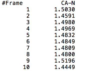
This command outputs a file that gives the distance from the center of mass of mask1 to the center of mass of mask2 at each time frame (mask1 and mask2 can either be residues or atoms). The output file will show two columns, one indicating the time frame number, and the other indicating the distance between the specified masks in Angstroms. The following visual shows a sample output of the command being called on the CA and N specified atoms (Carbon and Nitrogen respectively).

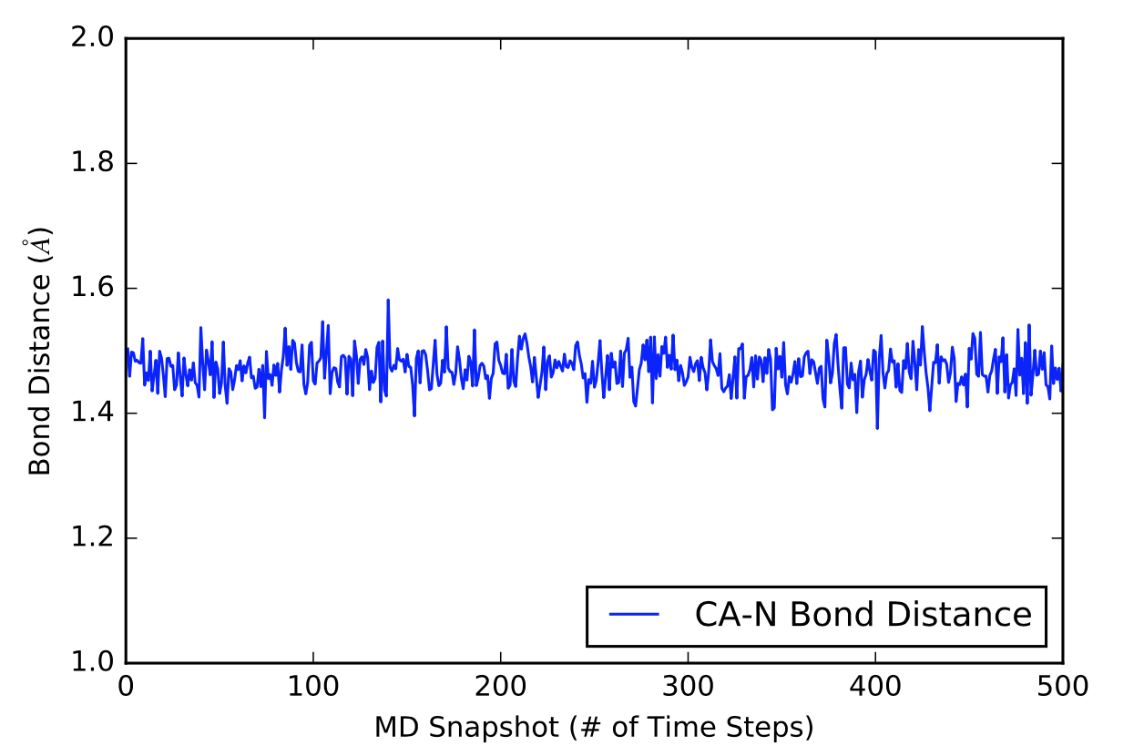
The next visual is a graph of the first 500 distance values in Angstroms in a 5000 time frame production run.

This action command can utilize other key modifiers to get slightly different outputs; however, the ones listed above are the main modifiers that are necessary to get decent data. When running CPPTRAJ on my production data on Melittin, the modifiers listed above were the only ones that I used.

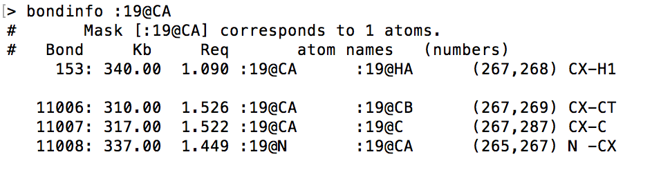
Example Usage: distance sample_name1 :19@CA :19@N out sample_data1.dat 


hbond [<name>] [out <filename>] [<mask>] [donormask <dmask> [donorhmask <dhmask>]] [solvout <filename>] [series [uvseries <filename>]]

This action command outputs a file that shows where there was hydrogen bonding in the molecule (or specified residue or atom). Some of these modifiers are not intuitively obvious and have yet to be seen in previous action commands, so below is the list of the modifiers that we have yet to identify in this post above and what they do.

  • [donormask <dmask> [donorhmask <dhmask]] refers to a specified residue or number of atoms that will be used as solute donor heavy atoms and a specified residue or number of atoms that will be used as solute donor hydrogen atoms respectively. The second mask should only be specified if the first mask is and the two masks should have a 1 to 1 correspondence between the two masks (in my case, one mask was specified as :WAT and the other was specified as :WAT@O, which represents the water box my Melittin was being simulated in).
  • [solvout <filename>] refers to the name of a file that will be outputted containing the averaged information of the solute-solvent hydrogen bonds in the specified [<mask>]. The output file will show the average distances and average angles of the hydrogen bonds formed between the acceptor and donor atoms (both of which are shown in the output file), along with the number of times a hydrogen bond formed and the fraction of the total number of hydrogen bonds that were specified by the [<mask>].
  • [series [uvseries <filename>]] refers to the name of a file that will be outputted containing the solute-solvent hydrogen bond time data in terms of whether a hydrogen bond was formed or not (as specified by a 1 meaning a hydrogen bond was formed, and a 0 meaning a hydrogen bond was not formed).

Normally, I would include sample data; however, the outputted data yielded very odd results that may or may not be completely useless, so I would much rather not give false data until I’m able to completely figure out how this command works. There are many other modifiers for this action command, but they turned out to be useless in my case.

Example Usage: hbond sample_name2 out sample_data2.dat solventdonor :WAT solventacceptor :WAT@O solvout sample_data3.dat series uvseries sample_data4.dat


rms/rmsd [<name>] <mask> [out <filename>]

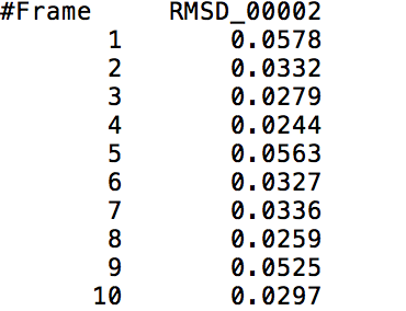
This action command outputs a file that contains the RMS Deviation values of a specified <mask> at each time frame. The following visual shows a small part of a sample output of the RMS Deviation values of the backbone of Tryptophan in Melittin.

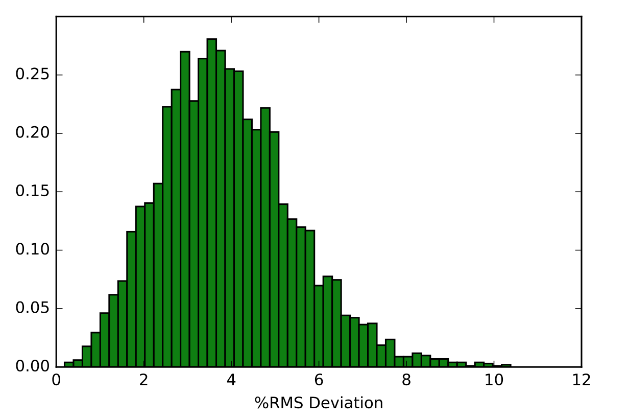
The next visual is a histogram of the 5000 RMS Deviation values that were outputted from using this command on the backbone of the Tryptophan in Melittin. The y-axis represents the fraction of RMS Deviation values that made up the data, while the x-axis represents the RMS Deviation values themselves.

Example Usage: rms sample_rms :19@C,CA,N out sample_rms.dat

Leave a Comment

Filed under chemistry, computing

Helpful CPPTRAJ Commands Part 1: Topology Commands

CPPTRAJ has a variety of commands for analyzing MD Simulation outputs, but because there are so many commands it would be very difficult to describe them all in detail in a single blogpost. As such, this first post will consist of the descriptions of three Topology Commands that I found to be useful for my research of the Tryptophan residue in Melittin. These Topology Commands print out Molecular Topology related information in CPPTRAJ’s interactive mode. For all intents and purposes, the visuals used in this blogpost will strictly be regarding Melittin.

Note: [<mask>] indicates a single residue/atom or range of residues/atoms


atominfo [<mask>]

This command prints out general information on each atom specified by the given [<mask>] modifier. The information is outputted into 12 columns. The following visual is an example output of the command being called on the 19th residue of a Melittin .mdcrd file.

  • #Atom refers to the atom’s index as given by Amber16
  • Name refers to the atom’s name identifier as given by Amber16
  • #Res refers to the residue number in which the atom is located
  • 2nd Name refers to the shorthand name of the residue in which the atom is located
  • #Mol refers to the atom’s molecule number
  • Type refers to the type of atom in the residue (i.e. alpha, beta, etc)
  • Charge refers to the electron charge of the atom
  • Mass refers to the mass of the atom
  • GBradius refers to the generalized Born radius of the atom
  • E1 refers to the element symbol
  • rVDW refers to the Van der Waal’s force radius of the atom
  • eVDW refers to the epsilon Van der Waal’s force of the atom

Example Usage: atominfo :19


bondinfo [<mask>]

This command prints out general information in the form of 6 columns about each bond between each atom as specified by the [<mask>] modifier. The following visual is an example output of the command being called on a specific carbon atom in the 19th residue of a Melittin .mdcrd file.

  • Bond refers to the bond index as specified by Amber16
  • Kb refers to the bond force constant
  • Req refers to the bond equilibrium value in Angstroms
  • atom names refers to the names of the bonded atoms as specified by Amber16
  • (numbers) refers to the atom indexes as specified by Amber16 as well as the types of atoms that are bonded together

Example Usage: bondinfo :19@CA


resinfo [<mask>]

This command prints out general information in 7 columns about a single residue or range of residues as specified by the given [<mask>] modifier. The following visual is an example output of this command being called on the range of residues that make up Melittin. The reason I had to indicate all the residues was because the .mdcrd file that I used had Melittin simulated in a water box. If the command was called without specifying the [<mask>] modifier, the output will include the residue info for all the water molecules in the water box as well. This goes for the atominfo and bondinfo commands too.

  • #Res refers to the residue index as specified by Amber16
  • Name refers to the shorthand name for each residue
  • First refers to the atom index of the first atom in the residue
  • Last refers to the atom index of the last atom in the residue
  • Natom refers to the number of atoms in the residue
  • #Orig refers to the original residue number in the original PDB file of which the date comes from
  • #Mol refers to the molecule number

One can also add the modifier, [short], to display the residues in the FASTA code sequence form. For Melittin, the sequence would look like this: GIGAVLKVLTTGLPALISWIKRKRQQ.

Example Usage: resinfo :1-26


Leave a Comment

Filed under chemistry, computing

A Look at Various Methods of Computationally Computing Absorbance Spectra

Yesterday was my senior seminar presentation.  I chose a paper entitled Computing the Absorption and Emission Spectra of 5-Methylcytidine in Different Solvents, which examined the absorbance spectra — and therefore also the vertical excitation energies — of a molecule called 5-methylcytidine in different solvents.  The authors (Martinez-Fernandez et. al.) use a range of solvation models and a mix of QM/MM/MD methods to find their spectra, and it is a fairly interesting look at different ways to computationally solve the problem.


In the paper, the absorption and emission spectra of 5-methylcytidine in water, acetonitrile, and tetrahydrofuran are studied both experimentally and computationally.  This molecule is chosen because it is the nucleoside associated with 5-methylcytosine, a derivative of the C base linked to UV caused mutations in DNA1,2.  The nucleoside is used instead of 5-methylcytosine itself because the sugar ring affects the absorbance and thus must be included for the results to be accurate to those of living systems.

When studying 5-methylcytidine, the paper seeks to answer two main questions: how the molecule’s spectra can be most accurately modelled computationally, and what insights into the solvent’s effects on the spectra can be found.  To answer these questions, the results of three computational methods were compared to experimental spectra.  In the first, the molecule was modelled using a static quantum mechanical approach, with the solvent being treated using a PCM model.  In the second, a static mixed quantum mechanical/molecular modelling approach is used, where the solvent-molecule interaction is initially simulated and optimized to a low energy point using MM, and then the absorption/emission energies are found using QM.  In the third, a molecular dynamics simulation is run, from which a sample of the different conformations of molecule and solvent are chosen.  The absorption/emission energies are then found at each of these points using MM single point calculations.  In each case, the absorption spectra obtained were stick spectra.  Over each peak, a Gaussian was fit to simulate vibrational effects and provide complete spectra.  Note for the emission spectra, only the first two methods were used as the third was computationally infeasible.

The computationally obtained absorption spectra all successfully predicted the three main peaks shown in the experimental spectra at 278 nm, 242 nm, 200 nm, though in some cases the peaks were blue shifted due to the lack of vibrational effects in the calculations.  Of the three computational methods, the third was most successful at predicting the experimental results, as it closely matched the experimental and included some absorbance between the two higher wavelength bands which the other models missed.  This was thought to likely be due to the increased accuracy of this method at representing the solvent.  The spectra also mirrored the solvent shifts seen in the experimental data, with acetonitrile and tetrahydrofuran having for the most part similar effects on the absorbance.  Their spectra relative to that of water were red shifted for the band at 278 nm and of higher intensity but similar energy for the other bands.

The computational emission spectra were consistent with those found experimentally for water.  The spectra of the other two solvents were similar to each other both experimentally and computationally.  For both solvents, the shift in the spectra from that of water were overestimated using both computational methods.  It was concluded that the main errors in both absorption and emission spectra were due to the lack of accounting for vibrational effects.

The differences in the absorption spectra for the solvents were concluded to be due to the hydrogen bonding ability of the solvent.  The HOMO and LUMO of the molecule in acetonitrile and tetrahydrofuran were very similar in shape and energy, despite the difference in polarity3 between the solvents.  This accounted for their similar absorbance, and suggested that solvent polarity is not the main factor in the solvent effect.  In water, hydrogen bonding dramatically changed the shapes of the HOMO and LUMO orbitals, thus changing their energies and the wavelengths which could be absorbed.  Therefore, hydrogen bonding was concluded to be the main cause of the solvent effects observed.


The paper can be found at:

Matrinez-Fernandez, L.; Pepino, A.; Segarra-Marti, J.; Banyasz, A.; Garavelli, M, Importa, R. Computing the Absorption and Emission Spectra of 5-Methylcytidine in Different Solvents: A Test-Case for Different Solvation Models.  Journal of Chemical Theory and Computation.  http://pubs.acs.org/doi/abs/10.1021/acs.jctc.6b00518?journalCode=jctcce


-Kristine

1 Comment

Filed under Paper Review

Molecular Dynamics Simulation Process and AMBER

I learned the Molecular Dynamics Simulation process by dealing with the protein Influenza Neuraminidase 3BEQ. Molecular Dynamics Simulation is a multi-step process.

First, I had to visit the protein data bank to download the protein Influenza Neuraminidase and put in a directory on comet. Second, I had to setup the protein in tleap in AMBER. While I set up the protein in tleap, I had to add Ions to the protein and solvate the system with a water box. Third, you have to save the protein in a coordinate and topology file. Fourth,  I needed to run energy minimizations using sander in AMBER. Fifth, I then needed to run equilibration. Sixth, I had to run a molecular dynamics run. Seventh, I had to use cpptraj to run a trajectory analysis. Lastly, I used VMD to view the simulation.

The process is tedious and allows a lot of place for error and typos, which could be annoying. Aside for the errors that could take place, the molecular dynamics simulation process is not too bad to handle with guidance.


2 Comments

Filed under chemistry

Using Putty and WinSCP to run molecular dynamics simulations on Influenza Neuraminidase 3BEQ

I first had to run a molecular dynamics simulation (via. workshop 1) to visualize the protein Influenza Neuraminidase 3BEQ. But before you can run a molecular dynamics simulation, you must know how to set up the simulation. Setting up the simulation and running the simulation wasn’t too bad. There is a learning curve when learning how to set up and run these simulations. All the errors I made when first trying to set up and run the simulation only helped me become better at the process.


I then had to run a molecular dynamics simulation (via workshop 2) to get the energy minimization and equilibration for the protein Influenza Neuraminidase 3BEQ. First time trying to run this simulation I encountered a road block, which was my own typos. Outside of the typos and making sure the input was perfect, I believe running these simulations was also not too bad. Errors also made me better at running this simulation.


Running these simulations through Putty introduced me to vim, which is a text editor. Vim allows you to edit a file in Putty. Learning Vim was not too bad also because of the Vim tutor that vim has. It teaches you the basics and everything I needed to know to successfully run the simulations.


The biggest thing I had to overcomer, for me, was to learn all these new features and remember how to use them. But once I surpassed the learning curve, It became progressively easier to get through the simulations.

1 Comment

Filed under computing