Category Archives: computing

A More In-Depth Look at the hbond Action Command in CPPTRAJ

As I have now accrued much more experience with CPPTRAJ and AMBER16 in general, I can now confidently explain more in-depth the hbond Action Command. While I still won’t be talking about every parameter of the hbond command (seeing as they’ve been explained for the most part in a previous blog post), I will be explaining a few of the other parameters that I did not mention in a previous blog post. As a review, the syntax is as follows:

hbond [<dsname>] [out <filename>] [<mask>] [angle <acut>] [dist <dcut>]

[donormask <dmask> [donorhmask <dhmask>]] [avgout <filename>]

[solvout <filename>] [series [uvseries <filename>]]

As I’ve already explained what some of these parameters do in a previous post, I will not explain what they do, rather, I will be explaining the parameters that you, the reader, have yet to see in this series of blog posts.

  • [angle <acut>] refers to the angle cutoff for hydrogen bond formation, meaning whatever the angle is set to, any hydrogen bond that forms at an angle smaller than what was specified, will not be counted as an actual hydrogen bond (CPPTRAJ ignores it). If this is not specified, then the default angle is 135 degrees. One can disable the cutoff by specifying the angle as -1.
  • [dist <dcut>] refers to the distance cutoff for hydrogen bond formation, meaning whatever the distance is set to, a hydrogen bond that forms with a bond length greater than the set distance will not be counted as an actual hydrogen bond (CPPTRAJ ignores it). If this is not specified, then the default distance is 3.0 Angstroms. One cannot disable this cutoff.
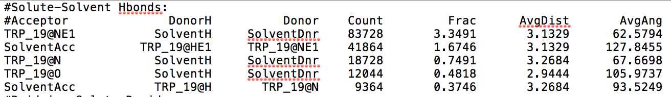
  • [avgout <filename>] refers to the name of a file that will be outputted containing information about the average bond length, the average bond angle, and the number of hydrogen bonds that formed throughout the entire production run for residues in which hydrogen bond formation happened.

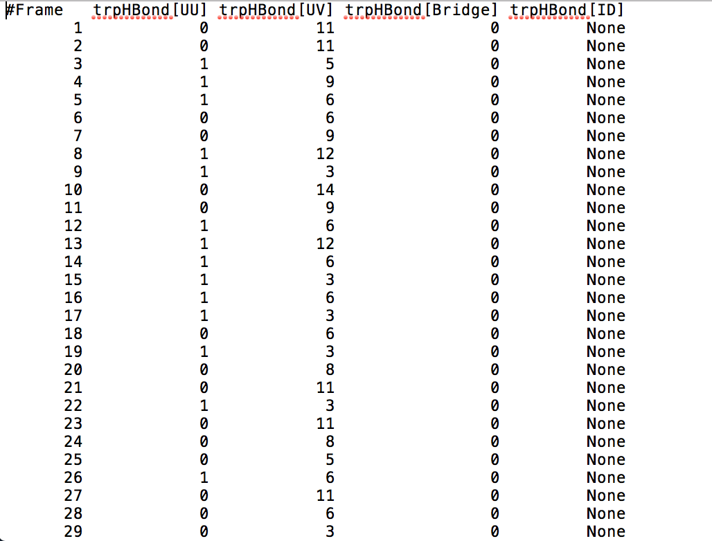
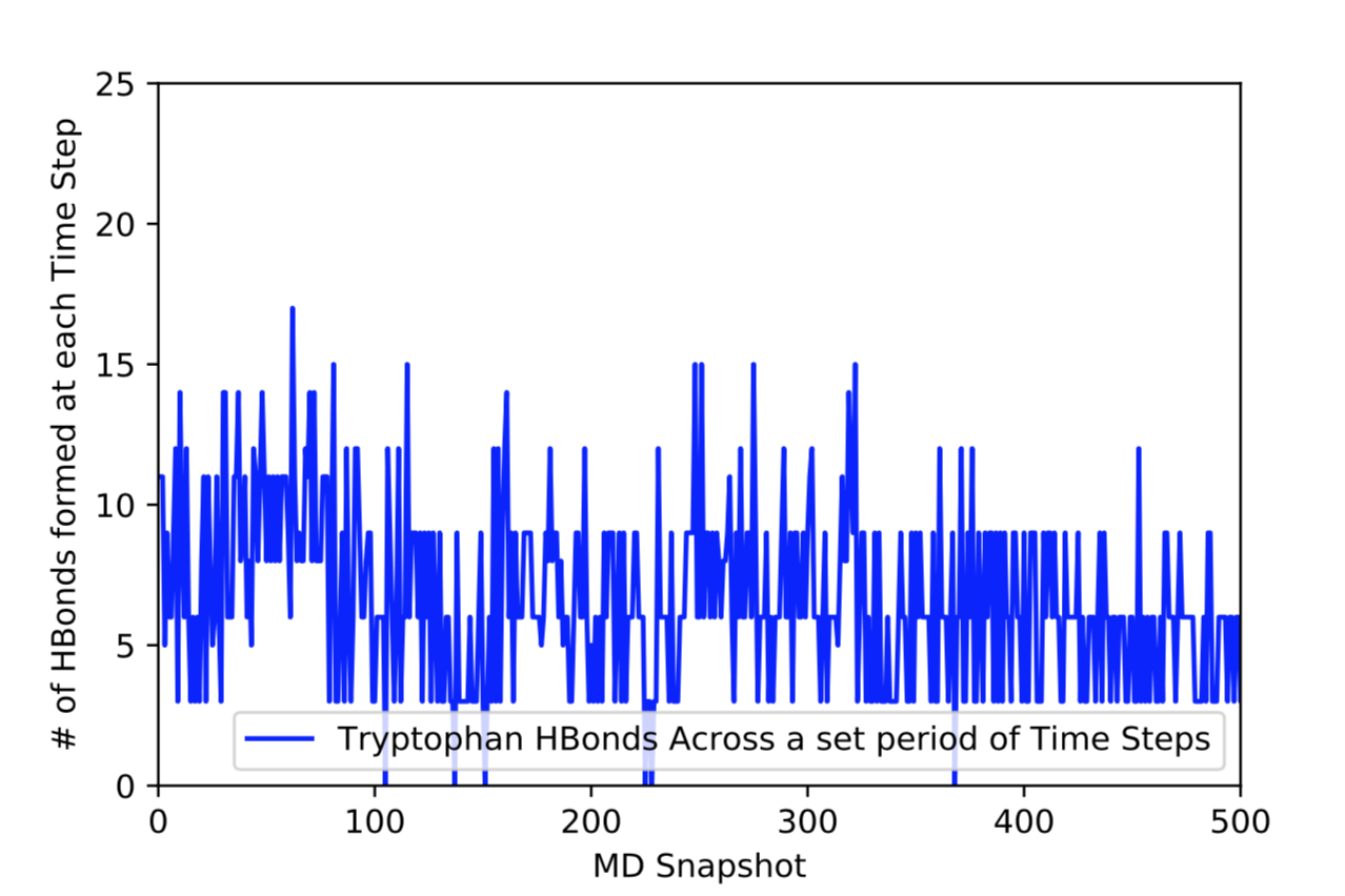
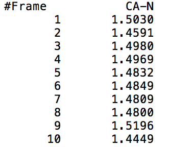
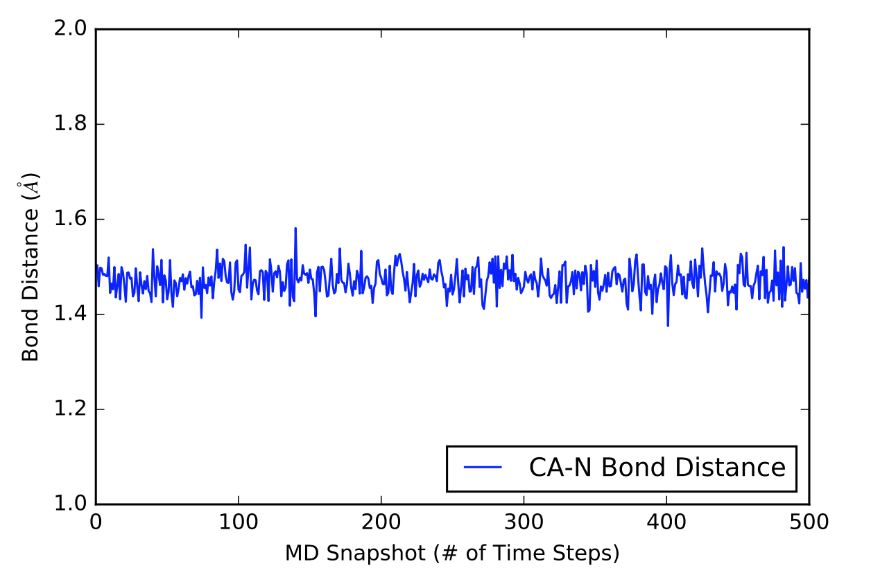
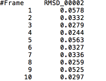
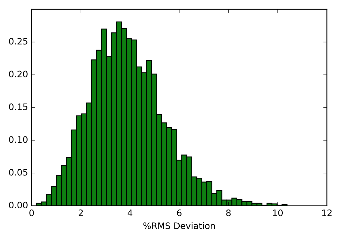
After learning about these parameters, I utilized them in my next production run, which yielded much more interesting results then the first time I used it. When I first used the hbond command, my results yielded nothing but 1’s and 0’s. That was because of the limiting default cutoffs. After disabling the angle cutoff and setting the distance cutoff to 3.5Å, my new data yielded much higher numbers. However, just because my data showed much better numbers, that doesn’t necessarily mean that many of those bonds can happen in real life. The reason those defaults are what they are is because those numbers are most likely the average lengths and angles in which hydrogen bonds actually form. Below are pictures of excerpts of the raw data, the average data, and a graph of the raw data of one of my production runs that utilized these new parameters. All of this data was obtained by doing a production run on the molecule, Melittin, and then by doing a trajectory run on the tryptophan of said Melittin. The exact syntax I used for the trajectory can be seen in the previous blog post (here is the link: http://williamkennerly.com/blog/a-mistake-with-the-hbond-action-command/)


1 Comment

Filed under chemistry, computing, programming

A Mistake with the hbond Action Command

In a previous blog post, I talked about how the hbond action command in CPPTRAJ is capable of outputting a file that shows whether or not a hydrogen bond formed across a series of time steps as indicated by a 1 or a 0 (for clarification, click on this link: http://williamkennerly.com/blog/helpful-cpptraj-commands-part-2-action-commands/). I recently found out that this is not entirely true. When I first used CPPTRAJ’s hbond command, the data I obtained only showed 0’s and 1’s in the solute-solvent hydrogen bond column. At the time, I had made the assumption that these 0’s and 1’s simply indicated whether or not hydrogen bonds formed at a certain time step, 0 meaning no hydrogen bonds were formed and 1 meaning one or more hydrogen bonds were formed. The reason my data yielded strange results was because of two things: a default angle cutoff for bond formation set at 135 degrees, and a default distance cutoff set at 3Å. These cutoffs meant that if a bond was to form at an angle smaller than 135 degrees or at a distance greater than 3Å, then CPPTRAJ does not count it and eliminates the data for that bond entirely.

After changing the cutoffs (I eliminated the angle cutoff by specifying the angle to be -1, and changed the distance cutoff to be 3.5Å), I obtained very different data. The following is the exact syntax that I used in my .traj file to get my output:

parm mlt_wat.prmtop

trajin mdcrd/prod.mdcrd

hbond trpHBond :19 out trp.HBvTime2.dat angle -1 dist 3.5 image solventdonor     :WAT solventacceptor :WAT@O solvout trp.HBAvg2.dat

run

quit

This .traj file uses a .mdcrd file that contains the final result of a production run of a whole Melittin molecule; however, by specifying the residue number (:19) I only extracted information about the hydrogen bonds formed with the respective tryptophan atoms that form them (the two Nitrogens and the Oxygen), which when plotted results in the graph seen at the bottom of this post. The problem with this obtained data is that it is most likely not reliable. While looking at the average angles of the hydrogen bonds, it was discovered that the angles were very acute ranging from 62° to 106°. They also had slightly longer bond lengths then the original cutoff of 3Å, the lengths ranging from 3 to 3.2Å. Therefore, it can be assumed that these bonds are unlikely to happen in nature.

1 Comment

Filed under chemistry, computing

Helpful CPPTRAJ Commands Part 2: Action Commands

The next three commands that I found to be helpful are known as Action Commands. Unlike the Topology Commands from the previous post, these Action Commands allow for a file to be created that contains the output. These commands can be used both in CPPTRAJ’s interactive mode, and in .ptraj files that can be called as inputs when starting CPPTRAJ.


distance [<name>] mask1 mask2 [out <filename>]

This command outputs a file that gives the distance from the center of mass of mask1 to the center of mass of mask2 at each time frame (mask1 and mask2 can either be residues or atoms). The output file will show two columns, one indicating the time frame number, and the other indicating the distance between the specified masks in Angstroms. The following visual shows a sample output of the command being called on the CA and N specified atoms (Carbon and Nitrogen respectively).

The next visual is a graph of the first 500 distance values in Angstroms in a 5000 time frame production run.

This action command can utilize other key modifiers to get slightly different outputs; however, the ones listed above are the main modifiers that are necessary to get decent data. When running CPPTRAJ on my production data on Melittin, the modifiers listed above were the only ones that I used.

Example Usage: distance sample_name1 :19@CA :19@N out sample_data1.dat 


hbond [<name>] [out <filename>] [<mask>] [donormask <dmask> [donorhmask <dhmask>]] [solvout <filename>] [series [uvseries <filename>]]

This action command outputs a file that shows where there was hydrogen bonding in the molecule (or specified residue or atom). Some of these modifiers are not intuitively obvious and have yet to be seen in previous action commands, so below is the list of the modifiers that we have yet to identify in this post above and what they do.

  • [donormask <dmask> [donorhmask <dhmask]] refers to a specified residue or number of atoms that will be used as solute donor heavy atoms and a specified residue or number of atoms that will be used as solute donor hydrogen atoms respectively. The second mask should only be specified if the first mask is and the two masks should have a 1 to 1 correspondence between the two masks (in my case, one mask was specified as :WAT and the other was specified as :WAT@O, which represents the water box my Melittin was being simulated in).
  • [solvout <filename>] refers to the name of a file that will be outputted containing the averaged information of the solute-solvent hydrogen bonds in the specified [<mask>]. The output file will show the average distances and average angles of the hydrogen bonds formed between the acceptor and donor atoms (both of which are shown in the output file), along with the number of times a hydrogen bond formed and the fraction of the total number of hydrogen bonds that were specified by the [<mask>].
  • [series [uvseries <filename>]] refers to the name of a file that will be outputted containing the solute-solvent hydrogen bond time data in terms of whether a hydrogen bond was formed or not (as specified by a 1 meaning a hydrogen bond was formed, and a 0 meaning a hydrogen bond was not formed).

Normally, I would include sample data; however, the outputted data yielded very odd results that may or may not be completely useless, so I would much rather not give false data until I’m able to completely figure out how this command works. There are many other modifiers for this action command, but they turned out to be useless in my case.

Example Usage: hbond sample_name2 out sample_data2.dat solventdonor :WAT solventacceptor :WAT@O solvout sample_data3.dat series uvseries sample_data4.dat


rms/rmsd [<name>] <mask> [out <filename>]

This action command outputs a file that contains the RMS Deviation values of a specified <mask> at each time frame. The following visual shows a small part of a sample output of the RMS Deviation values of the backbone of Tryptophan in Melittin.

The next visual is a histogram of the 5000 RMS Deviation values that were outputted from using this command on the backbone of the Tryptophan in Melittin. The y-axis represents the fraction of RMS Deviation values that made up the data, while the x-axis represents the RMS Deviation values themselves.

Example Usage: rms sample_rms :19@C,CA,N out sample_rms.dat

Leave a Comment

Filed under chemistry, computing

Helpful CPPTRAJ Commands Part 1: Topology Commands

CPPTRAJ has a variety of commands for analyzing MD Simulation outputs, but because there are so many commands it would be very difficult to describe them all in detail in a single blogpost. As such, this first post will consist of the descriptions of three Topology Commands that I found to be useful for my research of the Tryptophan residue in Melittin. These Topology Commands print out Molecular Topology related information in CPPTRAJ’s interactive mode. For all intents and purposes, the visuals used in this blogpost will strictly be regarding Melittin.

Note: [<mask>] indicates a single residue/atom or range of residues/atoms


atominfo [<mask>]

This command prints out general information on each atom specified by the given [<mask>] modifier. The information is outputted into 12 columns. The following visual is an example output of the command being called on the 19th residue of a Melittin .mdcrd file.

  • #Atom refers to the atom’s index as given by Amber16
  • Name refers to the atom’s name identifier as given by Amber16
  • #Res refers to the residue number in which the atom is located
  • 2nd Name refers to the shorthand name of the residue in which the atom is located
  • #Mol refers to the atom’s molecule number
  • Type refers to the type of atom in the residue (i.e. alpha, beta, etc)
  • Charge refers to the electron charge of the atom
  • Mass refers to the mass of the atom
  • GBradius refers to the generalized Born radius of the atom
  • E1 refers to the element symbol
  • rVDW refers to the Van der Waal’s force radius of the atom
  • eVDW refers to the epsilon Van der Waal’s force of the atom

Example Usage: atominfo :19


bondinfo [<mask>]

This command prints out general information in the form of 6 columns about each bond between each atom as specified by the [<mask>] modifier. The following visual is an example output of the command being called on a specific carbon atom in the 19th residue of a Melittin .mdcrd file.

  • Bond refers to the bond index as specified by Amber16
  • Kb refers to the bond force constant
  • Req refers to the bond equilibrium value in Angstroms
  • atom names refers to the names of the bonded atoms as specified by Amber16
  • (numbers) refers to the atom indexes as specified by Amber16 as well as the types of atoms that are bonded together

Example Usage: bondinfo :19@CA


resinfo [<mask>]

This command prints out general information in 7 columns about a single residue or range of residues as specified by the given [<mask>] modifier. The following visual is an example output of this command being called on the range of residues that make up Melittin. The reason I had to indicate all the residues was because the .mdcrd file that I used had Melittin simulated in a water box. If the command was called without specifying the [<mask>] modifier, the output will include the residue info for all the water molecules in the water box as well. This goes for the atominfo and bondinfo commands too.

  • #Res refers to the residue index as specified by Amber16
  • Name refers to the shorthand name for each residue
  • First refers to the atom index of the first atom in the residue
  • Last refers to the atom index of the last atom in the residue
  • Natom refers to the number of atoms in the residue
  • #Orig refers to the original residue number in the original PDB file of which the date comes from
  • #Mol refers to the molecule number

One can also add the modifier, [short], to display the residues in the FASTA code sequence form. For Melittin, the sequence would look like this: GIGAVLKVLTTGLPALISWIKRKRQQ.

Example Usage: resinfo :1-26


Leave a Comment

Filed under chemistry, computing

Running the NewtonX Tutorial

After I got the tests to run, I started working my way through the tutorial.  Specifically, I am trying part 4.  I managed to get to step 18 before I ran into problems.  In step 18, we are trying to generate the inital conditions for NewtonX to use.  To do this you run a line of code:

$NX/initcond.pl >initcond.log &

This line of code immediately spits out a message which is a number in brackets followed by another number.  The numbers change each time.  It then prints a message saying initcond.pl is dying now.  At this point, the console freezes and does not respond until you abort with ctrl-c.  It then spits out an exit code, “Exit 255.” (Which I have been unable to find more information on).

To try to figure out what was wrong, I examined the initcond.log file.  So far I have gotten two different messages which seem to alternate with no real reason.  The first occurs early in the run and says:

Cheking input files

Cheking geometry lines

Searching for qvector...

qvector does not exist

Creating qvector...

It appears to die while trying to make the missing qvector.  The qvector it is referring to used to be a file in version 1.1 that contained the quantum vibrational number, but it isn’t referenced at all in 1.4.

The second error happens later in the run and says:

Starting run_g09_initcond.pl at Tue Nov 22 08:21:30 PST 2016

Vertical energies with Gaussian 09

Starting .  $g09root/g09/bsd/g09.profile;$g09root/g09/g09 gaussian.com at Tue Nov 22 08:21:30 PST 2016

Finished .  $g09root/g09/bsd/g09.profile;$g09root/g09/g09 gaussian.com with ERROR at Tue Nov 22 08:21:30 PST 2016

Finished run_g09_initcond.pl with ERROR at Tue Nov 22 08:21:30 PST 2016

This error seems to be referring to the same issue with NewtonX inserting an extra /g09/ which we were seeing earlier.  However, when I tried using the same set of variable definitions which worked in the tests, it did not change anything.  Also, I poked around in the file and found the same qvector error as earlier but instead of crashing after creating the qvector, it continued successfully.  So it seems like that error is one that it can sometimes get past.

So far I haven’t been able to figure out when one error occurs versus the other.  There doesn’t seem to be any particular logic to it.

-Kristine


2 Comments

Filed under computing

Running the NewtonX Tests

First you need to install NewtonX.  To do this, you request a download link from the NewtonX site, follow the link, and download the binary file recommended (it will be called something like “NX-1.4.0-3-source+binary.tgz”).  Then copy the file to comet, and untar and unzip it by typing tar -zxf NX-1.4.0-3-source+binary.tgz.  This corresponds to section 9.1 in the documentation.  Do not go further and do 9.2; 9.2 is only for if you want to install the program manually.

After installing NewtonX, I spent a while trying to get the built in tests to run.  Eventually I came up with this procedure:

First we have to set up the variables so NewtonX can find Gaussian.  We do this through the following lines of code:

export NX=/home/kvorwerk/NX-1.4.0-2/bin
export g09root=/share/apps/compute/gaussian/09.E.01/g09
source $g09root/bsd/g09.profile
export g09root=/share/apps/compute/gaussian/09.E.01

The last line is necessary to avoid an error by which NewtonX adds an extra /g09/ into the path where it searches for gaussian.  Also note the line setting the NX variable would need to be modified to match the path where you installed NewtonX.

Next we make a directory to run the tests in.  This can be anywhere.  Then we select the tests to run by typing:

$NX/inp-testnx.pl

This shows a list of tests.  We want to run the gaussian09 one and the NewtonX ones; that is, 18, 19, 24, and 25.  To actually run the tests we type:

$NX/test-nx.pl >test.log

This creates a bunch of subdirectories and a file called test.log.  The test.log file contains basic output, and more output is in the sub directories.  When I ran the tests, the test.log file told me that:

18 finished, but with a message saying:

Files /home/kvorwerk/nx_test/TEST_NX/MD-SICH4-G09-TDDFT-NAD/RESULTS/dyn.out and   /home/kvorwerk/NX-1.4.0-2/bin/../test-nx/STANDARD-RESULTS/MD-SICH4-G0    9-TDDFT-NAD/RESULTS/dyn.out differ.  It seems to be important differences. Something may be wrong in the installation.

The files it refers to are easy to find.  However, I have been unable to find the file or script which compared them.

19 finished normally

24 finished with a message saying:

Files /home/kvorwerk/nx_test/TEST_NX/MD-ANALYTICAL-MODEL1/RESULTS/dyn.out and   /home/kvorwerk/NX-1.4.0-2/bin/../test-nx/STANDARD-RESULTS/MD-ANALYTIC    AL-MODEL1/RESULTS/dyn.out differ.  It seems to be only minor numerical differences. Probably installation is OK.

I do not think this error is worth worrying about.

25 finished normally.

The issue with test 18 may be due to us using a more recent version of gaussian (09.E) than the developers used to create the test.  Hopefully we will be able to find the comparisson they use and learn if this is indeed the case.

-Kristine

1 Comment

Filed under computing

Errors Galore

I have been having to process and handle a wide variety of errors in the past few weeks, using Gaussian as well as Comet. Here are the conclusions we found if you ever run into similar errors.

  1. FileIO error:   This error was quite odd and took a lot of work to surpass. It was seen in at least three excited state optimization calculation output files but there was no other trend visible based on functional, basis set, or root number. This image is difficult to read but it essentially is a very long list of groups of numbers (like at the top), followed by “dumping /fiocom/ . . .  . . Ntrerr called from FileIO”. After communicating with Gaussian Tech Support, they offered the advice of updating our Gaussian to the E version. To do this, go to the gaussian.sh file and where it says “module load gaussian,” correct it to “module load gaussian.09.E.01” and save. This error was due to a bug in the older version that we had been using, although it could have been circumvented using “opt=nolinear” or “guess=always” as a keyword. For this reason, we have been using version E of Gaussian for all further calculations. FileIO
  2. Python plots: In the energy_step_oscillator_plot.py script, I had difficult writing to the results file. Whenever I would run the module, the correct plot would pop up but then the results file would be empty (blank and 0KB). To see the proper results, make sure to refresh the folder in which the results.txt file is and also close the plot before opening the results. This is necessary if and only if your script reads to “results.close()” AFTER the plot order. If you simply move “results.close()” to before the plot instructions, this will not be an issue. Now, the results.txt file will close before the plots are displayed.
  3. There have been multiple different cases where jobs on comet required more memory. There would be a message towards the end of the prematurely terminated output file asking for more MW, which is a different unit of memory storage. I have been adding “%Mem=8GB” to almost all of my input .gjf files (as the first line) to ensure that the job doesn’t end early.
  4. If a job terminates otherwise but there is no clear explanation, this probably indicates that there was not enough wall time to perform the calculation entirely, so you should add more wall time or increase the number of processors you use for the calculation. To do so, you must change “nprocshared=1” to “nprocshared=8” and “ntasks-per-node=1” to “ntasks-per-node=8” or any number between 1 and 8, and also include “%nprocshared=#” at the top of your input file. This can show a dramatic decrease in the time necessary to perform certain calculations.

1 Comment

Filed under computing

Decoding: AMBER code

In a previous blog post, I presented a code I used in AMBER to run a trajectory of a protein. The code is below:

nohup mpirun -np 4 sander.MPI -O -i mdin -p 3beq.top -c 3beq.crd -r 3beq_md.crd -x md.trj -o md.out &

Before you can run code successfully, you have to know what the code means and how to set up the code. The code above contains flags and the files you need to run the simulation. The flags precede the files that contribute to the flags. The flags are the individual letters with the dash in front of them.

Flags:

  • -O: overwrites any output file with the same name
  • -i: input file
  • -p: parmtop file
  • -c: coordinate file
  • -r: restart file (output of new coordinates)
  • -x: trajectory file
  • -o: output file
  • -np: specifies the number of processors
  • -ref: reference file [Not in code above, but used in other codes]

Other than the flags and files, there are commands that also contribute to the running of the code. The command nohup and & are used. As previously discussed, nohup allows codes to run without hanging up and & allows codes to run in the background. So together, nohup and &, allows you to logout of comet or continue doing other things on comet while your job runs. A new command that is present in the code is mpirun, which cause the code to be executed in parallel.

1 Comment

Filed under computing

Using Vi/Vim

Vi and Vim are ultimately the same thing. Vim is just the improved version of Vi. Vi/Vim is a text editor that is used in PuTTY when using comet.

Vim is needed when running molecular dynamics simulations because it allows you to quickly edit files and check results in output files. But, Vim isn’t your average text editor. Since it is designed for software like PuTTY, it makes editing very easy. The easy editing and the ability to edit your files in any way makes Vim very powerful.

Vim has many commands that contribute to how powerful the text editor is. Some of the helpful commands in Vim are :wq, i, u, G, gg, and :help cmd. Command, :wq, saves all the edits you have done to the file. Command, i, enables insert mode, which allows you to insert and delete things. Command, u, undoes previous action. Command, G, moves to the  end of the file. Command, gg, moves to the beginning of the file. Command, :help cmd, gives you help about whatever cmd is. cmd can be anything you need help with.

One amazing thing about Vim that is helpful and essential is vimtutor. Vimtutor is a multi-lesson tutorial on how to use and gives you important commands to use Vim. Each lesson have many parts to it. If you go through the entire tutorial, you will be about to effectively use Vim. There is a learning curve though. It takes a while to get use to, but after practice with Vim and using Vim, you’ll be a pro.

Vim

Above is the beginning of vimtutor.


1 Comment

Filed under computing

Accessing and Using Comet

Comet is the super computer center in San Diego that I’m using to run molecular dynamics simulations. In order to use the super computer in San Diego on your local computer, you have to use a ssh client and a scp client. Since I am wirking on a Windows computer, the ssh client I used was PuTTY and the scp client I used was WinSCP. There are different programs to use on other operating systems. All you have to do is sign into your comet account on PuTTY and WinSCP, and you have access to the things in your comet account and the super computer.

The ssh client, PuTTY, is the program that allows you to communicate directly to the super computer. PuTTY on your local computer connects the remote computer, comet. When you are typing in and navigating PuTTY, you are typing in and navigating comet. The actual molecular dynamics simulations are done in PuTTY.

The scp client, WinSCP, is the program that allows you to transfer files from comet to your local computer. You can easily transfer files back and forth, from local to emote computer in a short period of time.

To learn how to use comet, I had to learn how to use PuTTY and WinSCP. Also, I needed to learn basic linux commands because in PuTTY you use linux commands to control comet. Linux commands like mkdir, cd, cp, mv, and ls are really essential and used a lot. mkdir creates a directory, cd changes the directory, cp copies files, mv moves files, and ls lists the files in the current directory. I think the nohup command followed by the & at the end of job was most useful so far because it allows jobs to run in the background without hanging up. This allows you to run other jobs or do other things without stopping the job. WinSCP can be used like any other file manager program, no linux commands needed.

An example of the nohup command to run a trajectory:
nohup mpirun -np 4 sander.MPI -O -i mdin -p 3beq.top -c 3beq.crd -r 3beq_md.crd -x md.trj -o md.out &

Comet allows me access to AMBER, which lets me use tleap, sander, and cpptraj. Those are programs are essential to running molecular dynamics.

PuTTY and WinSCP

Comet is the black screen on the left and WinSCP is the left screen.

2 Comments

Filed under computing