Author Archives: Alexandra Cassell

MERCURY Conference

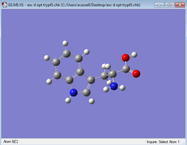
I really enjoyed going to this year’s MERCURY conference. In fact, a few of the speakers were very inspirational, as were some posters. The speakers that I most enjoyed were Kate Holloway and Chris Wilmer. Kate Holloway talked about drug design to combat HIV and HCV and I was really intrigued by the details and difficulties in this process. Chris Wilmer discussed MOF’s and how they can be used to model methane consumption. I think I liked these presentations the most, both because the speakers were very good and also because I could clearly see the applications of their research in our lives. I also really enjoyed the poster session. My presentation went well, except I was asked a few questions I was uncertain about and Chris Cramer didn’t come to talk to me 🙁 . However, I enjoyed looking at other posters more than presenting my own. There were three posters that I enjoyed the most. First, a student researched nano-aggregates and measured their speed of aggregation to be able to find a solution to clogging when these nano-aggregates interact with waxes in pipes. Her research seemed very simple on the poster, but the work was quite fascinating. Second, a student experimented with different halogens and leaving groups to see if he could make a bi-molecular reaction become a concerted reaction. I don’t think I realized how many different directions molecular dynamics could go; including organic chemistry. Lastly, two girls presented their poster about enzyme inhibitors. I can’t quite remember the entire purpose but I know that they were working with inhibitors, derivatives of some molecule (which included tryptophan), and dopamine. They measured interaction energies between the derivatives and dopamine to find the best one, with two different conformations.

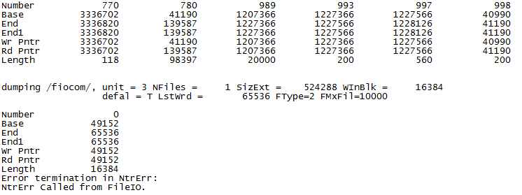
I was disappointed that I wasn’t able to get any suggestions about Gaussian’s confusion problem from any of the quantum professors or speakers there who are familiar with the program. I would have liked to been able to discuss more with them the problems that we have been  having. Overall, I enjoyed seeing the subjects that other students were researching with computational chemistry. Also, the conference made me sad that I am not taking a science class next semester. . .

1 Comment

Filed under conference report

Errors Galore

I have been having to process and handle a wide variety of errors in the past few weeks, using Gaussian as well as Comet. Here are the conclusions we found if you ever run into similar errors.

  1. FileIO error:   This error was quite odd and took a lot of work to surpass. It was seen in at least three excited state optimization calculation output files but there was no other trend visible based on functional, basis set, or root number. This image is difficult to read but it essentially is a very long list of groups of numbers (like at the top), followed by “dumping /fiocom/ . . .  . . Ntrerr called from FileIO”. After communicating with Gaussian Tech Support, they offered the advice of updating our Gaussian to the E version. To do this, go to the gaussian.sh file and where it says “module load gaussian,” correct it to “module load gaussian.09.E.01” and save. This error was due to a bug in the older version that we had been using, although it could have been circumvented using “opt=nolinear” or “guess=always” as a keyword. For this reason, we have been using version E of Gaussian for all further calculations. FileIO
  2. Python plots: In the energy_step_oscillator_plot.py script, I had difficult writing to the results file. Whenever I would run the module, the correct plot would pop up but then the results file would be empty (blank and 0KB). To see the proper results, make sure to refresh the folder in which the results.txt file is and also close the plot before opening the results. This is necessary if and only if your script reads to “results.close()” AFTER the plot order. If you simply move “results.close()” to before the plot instructions, this will not be an issue. Now, the results.txt file will close before the plots are displayed.
  3. There have been multiple different cases where jobs on comet required more memory. There would be a message towards the end of the prematurely terminated output file asking for more MW, which is a different unit of memory storage. I have been adding “%Mem=8GB” to almost all of my input .gjf files (as the first line) to ensure that the job doesn’t end early.
  4. If a job terminates otherwise but there is no clear explanation, this probably indicates that there was not enough wall time to perform the calculation entirely, so you should add more wall time or increase the number of processors you use for the calculation. To do so, you must change “nprocshared=1” to “nprocshared=8” and “ntasks-per-node=1” to “ntasks-per-node=8” or any number between 1 and 8, and also include “%nprocshared=#” at the top of your input file. This can show a dramatic decrease in the time necessary to perform certain calculations.

1 Comment

Filed under computing

Different Basis Sets for Gaussian Calculations

There are multiple types of functionals and basis sets that can be used for different calculations in Gaussian such as optimizations, scans, and excited state energy calculations. A basis set is a set of basis functions. Each basis set is a different size and generally, the bigger the basis set size, the more accurate the results will be. The names of the basis sets accessible through Gaussian are 6-31G (which can include +,++, and different orbitals), STO-3G, 3-21G, 6-311G, cc-pVDZ, cc-pVTZ, cc-pVQZ, LanL2DZ, LanL2MB, SDD, DGDZVP, DGDZVP2, DGTZVP, GEN, and GENECP. However, really there are many more options available which are discussed more thoroughly on the following website (http://www.gaussian.com/g_tech/g_ur/m_basis_sets.htm). It is also possible to create your own basis set using Gaussian, but this can be time-consuming and complicated. In relation to 6-31G, the increasing size of the basis set in terms of +, ++, aug- (which are augmented basis sets)  and p,d,f orbitals or *,** (polarization functions), the more that are included, the more accurate results these should be as well. Each basis set contains a different number of Cartesian (etc) basis functions, which can be found in the output file (ctrl-f “basis function”). The larger the number of basis functions corresponds to a longer calculation time.

I performed an optimization calculation on a new conformation of tryptophan and then ran excited state calculations using 16 combinations of functionals (b3lyp, cam-b3lyp, pbepbe, and wb97xd) and basis sets (6-31G, 6-31+G, 6-31+G(d,p), and cc-pVDZ). Since 6-31G is the smallest basis set here, it took the shortest time to complete calculations in all of the functionals. Also, within functionals, cc-pVDZ is similar in time to 6-31G. Below is a table showing the times and number of basis functions for each basis set that was used in calculating excited state energies of an optimized configuration of tryptophan.

A) Basis set: 6-31G

Cartesian Basis functions: 159

Functional b3lyp cam-b3lyp PBEPBE wB97XD
Job CPU Time / Minutes 7.733 9.717 7.45 10.1


B) Basis set: 6-31+G

Cartesian Basis functions: 219

Functional b3lyp cam-b3lyp PBEPBE wB97XD
Job CPU Time / Minutes 25.88 34.63 20.5 34.65


C) Basis set: 6-31+G(d,p)

Cartesian Basis functions: 345

Functional b3lyp cam-b3lyp PBEPBE wB97XD
Job CPU Time / Minutes 59.53 76.0167 48.05 81.783


D) Basis set: cc-pvdz

Cartesian basis functions: 285

Functional b3lyp cam-b3lyp PBEPBE wB97XD
Job CPU Time / Minutes 29.0167 39.267 24.6 39.03


2 Comments

Filed under computing

How to Visualize Molecular Orbitals on GaussView

Open GaussView and click File->Open…, then open a checkpoint (.chk) files. After the GaussView image appears like below, click from the toolbar Results->Surfaces/Contours..

image (4)image (1)

A new window will open. Select the Cube Actions dropdown and click New Cube. Make sure that the top “Type” dropdown is set to Molecular Orbital. Here, you can choose what type of molecular orbital you would like to illustrate (under the HOMO dropdown). For example, the options include HOMO, LUMO, Occupied, Virtual, or you can choose your own combination or molecular orbitals by number. Once you choose, click OK. Then, click the Surface Actions dropdown and click New Surface. This will add the MO’s to your GaussView image.

Below are representations of the HOMO and LUMO molecular orbitals of one conformation of tryptophan.

image (2)image (3)

Leave a Comment

Filed under chemistry

Trp Geometry Optimization Calculations with Gaussian

Optimization calculations are not too difficult. However, challenges can arise as can many different results. I did an optimization on three different conformations of tryptophan that I created by changing one of many dihedral angles in the molecule (Two C’s in pentagon across from N, the next Carbon in substituent chain, and the next Carbon which was bonded to NH2).

image

I used angles of 0, 135, and 180 degrees. Using the “broom”/”sweep” button on GaussView, I was able to return each configuration to a more energetically favorable conformation near those angles (21.99, -158.0, 41.5, respectively). However, they were not all the same since these angles are quite far from one another. When I performed an optimization calculation, each gave very similar energies (within 2 kJ/mol; in fact the first and third configuration were the same up to the fourth decimal place), but ranged in their change in energy from the “swept” conformation.

Here comes the issue. One calculation would not run (B3LYP/6-31G). It failed three times, each 15 minute long trials. The error message overall read “Error with lnk1e” followed by another line of error (which I do not remember). This suggested that the error arose because the “redundant internal coordinates” of this optimization were not working. So, one method to fix this issue would be to run the calculation starting from the current coordinates in the checkpoint file to redefine the internal coordinates and essentially bypass the error. Yet, in one of the output images, one C-C bond was essentially broken which shows that in its attempt to optimize the energy of tryptophan, GaussView felt that these two atoms needed to be further apart (about 1.75 Angstroms) than a normal C-C bond (1.54 A). This is not a scenario that should be repeated so the method of starting with new coordinates from the checkpoint file would not be effective. Therefore, instead we decided to use Cartesian coordinates which required adding “opt=cartesian” into the keywords of the route line.

Although a cartesian calculation takes much longer, I was able to find the proper energy of the optimized molecule.


1 Comment

Filed under chemistry