Tag Archives: Gaussian

Python Error-Handling: Follow-up to Temporary Files

This post is a follow-up to this previous blog post.

On the new Windows 10 computers at Skidmore, I ran into the issue when running python in which temporary files disrupt the execution of my scripts. An example of a suspected temporary file is “C:\Users\jgerard\Desktop\Important2\~$LYP-D_root1.gjf.out”. However, when I select “View Hidden Files” in my directory, no such file appears. As a last resort, I have my script search for temporary files:

if "$" in file_name:

and break if True. This adjustment allowed the successful run of the script. However, it is less than elegant, and the script could run into issues if any of my output files were to include a “$” in their file name.

Leave a Comment

Filed under programming

A Look at Various Methods of Computationally Computing Absorbance Spectra

Yesterday was my senior seminar presentation.  I chose a paper entitled Computing the Absorption and Emission Spectra of 5-Methylcytidine in Different Solvents, which examined the absorbance spectra — and therefore also the vertical excitation energies — of a molecule called 5-methylcytidine in different solvents.  The authors (Martinez-Fernandez et. al.) use a range of solvation models and a mix of QM/MM/MD methods to find their spectra, and it is a fairly interesting look at different ways to computationally solve the problem.


In the paper, the absorption and emission spectra of 5-methylcytidine in water, acetonitrile, and tetrahydrofuran are studied both experimentally and computationally.  This molecule is chosen because it is the nucleoside associated with 5-methylcytosine, a derivative of the C base linked to UV caused mutations in DNA1,2.  The nucleoside is used instead of 5-methylcytosine itself because the sugar ring affects the absorbance and thus must be included for the results to be accurate to those of living systems.

When studying 5-methylcytidine, the paper seeks to answer two main questions: how the molecule’s spectra can be most accurately modelled computationally, and what insights into the solvent’s effects on the spectra can be found.  To answer these questions, the results of three computational methods were compared to experimental spectra.  In the first, the molecule was modelled using a static quantum mechanical approach, with the solvent being treated using a PCM model.  In the second, a static mixed quantum mechanical/molecular modelling approach is used, where the solvent-molecule interaction is initially simulated and optimized to a low energy point using MM, and then the absorption/emission energies are found using QM.  In the third, a molecular dynamics simulation is run, from which a sample of the different conformations of molecule and solvent are chosen.  The absorption/emission energies are then found at each of these points using MM single point calculations.  In each case, the absorption spectra obtained were stick spectra.  Over each peak, a Gaussian was fit to simulate vibrational effects and provide complete spectra.  Note for the emission spectra, only the first two methods were used as the third was computationally infeasible.

The computationally obtained absorption spectra all successfully predicted the three main peaks shown in the experimental spectra at 278 nm, 242 nm, 200 nm, though in some cases the peaks were blue shifted due to the lack of vibrational effects in the calculations.  Of the three computational methods, the third was most successful at predicting the experimental results, as it closely matched the experimental and included some absorbance between the two higher wavelength bands which the other models missed.  This was thought to likely be due to the increased accuracy of this method at representing the solvent.  The spectra also mirrored the solvent shifts seen in the experimental data, with acetonitrile and tetrahydrofuran having for the most part similar effects on the absorbance.  Their spectra relative to that of water were red shifted for the band at 278 nm and of higher intensity but similar energy for the other bands.

The computational emission spectra were consistent with those found experimentally for water.  The spectra of the other two solvents were similar to each other both experimentally and computationally.  For both solvents, the shift in the spectra from that of water were overestimated using both computational methods.  It was concluded that the main errors in both absorption and emission spectra were due to the lack of accounting for vibrational effects.

The differences in the absorption spectra for the solvents were concluded to be due to the hydrogen bonding ability of the solvent.  The HOMO and LUMO of the molecule in acetonitrile and tetrahydrofuran were very similar in shape and energy, despite the difference in polarity3 between the solvents.  This accounted for their similar absorbance, and suggested that solvent polarity is not the main factor in the solvent effect.  In water, hydrogen bonding dramatically changed the shapes of the HOMO and LUMO orbitals, thus changing their energies and the wavelengths which could be absorbed.  Therefore, hydrogen bonding was concluded to be the main cause of the solvent effects observed.


The paper can be found at:

Matrinez-Fernandez, L.; Pepino, A.; Segarra-Marti, J.; Banyasz, A.; Garavelli, M, Importa, R. Computing the Absorption and Emission Spectra of 5-Methylcytidine in Different Solvents: A Test-Case for Different Solvation Models.  Journal of Chemical Theory and Computation.  http://pubs.acs.org/doi/abs/10.1021/acs.jctc.6b00518?journalCode=jctcce


-Kristine

1 Comment

Filed under Paper Review

Python Error Handling: Temporary Files and Skipping Failed Jobs

In my scripts that analyze all Gaussian output files in a directory, I use glob to get all the files into a list. The relevant script is as follows:

import glob

#get a folder to search through
folder_location = get_folder_location()

#gets filepaths for everything in the specified folder ending with .LOG or .out
search_str_log = folder_location + "*.LOG"
search_str_out = folder_location + "*.out"

file_paths_log = glob.glob(search_str_log)
file_paths_out = glob.glob(search_str_out)

file_paths = file_paths_log + file_paths_out

I have been editing and testing output files within the directory, and my script has mistakenly read their temporary Word files as .out files. I needed to make those temporary files visible (see this link for instructions on how to do that). Then I deleted the temporary files, so they would not be read as extra files.


I wanted my script to skip files that had in error termination in Gaussian, so I needed to search the output files for the string “Error termination”. Since I was reading output files with .readlines(), as a list of lines (strings), I decided to recombine the list of strings into one string as follows:

#reads the file as a list of its lines of text
content_lines = current_file.readlines()

combined = '\t'.join(content_lines)

if "Error termination" in combined:
    print file_name + " skipped because of error termination
    in Gaussian."

else:
    #analyze file

Another option would have been to use .read() in addition to .readlines() for a different variable content, but that would set the cursor to the end of the file, and I would need to write current_file.seek(0) to reset the cursor to the beginning of the file. (See this post for more information about this issue.) Using the .join() command was a simpler way of getting the text file as a string, without having to set the cursor back.

2 Comments

Filed under programming

Errors Galore

I have been having to process and handle a wide variety of errors in the past few weeks, using Gaussian as well as Comet. Here are the conclusions we found if you ever run into similar errors.

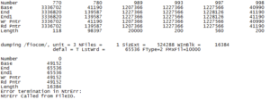
  1. FileIO error:   This error was quite odd and took a lot of work to surpass. It was seen in at least three excited state optimization calculation output files but there was no other trend visible based on functional, basis set, or root number. This image is difficult to read but it essentially is a very long list of groups of numbers (like at the top), followed by “dumping /fiocom/ . . .  . . Ntrerr called from FileIO”. After communicating with Gaussian Tech Support, they offered the advice of updating our Gaussian to the E version. To do this, go to the gaussian.sh file and where it says “module load gaussian,” correct it to “module load gaussian.09.E.01” and save. This error was due to a bug in the older version that we had been using, although it could have been circumvented using “opt=nolinear” or “guess=always” as a keyword. For this reason, we have been using version E of Gaussian for all further calculations. FileIO
  2. Python plots: In the energy_step_oscillator_plot.py script, I had difficult writing to the results file. Whenever I would run the module, the correct plot would pop up but then the results file would be empty (blank and 0KB). To see the proper results, make sure to refresh the folder in which the results.txt file is and also close the plot before opening the results. This is necessary if and only if your script reads to “results.close()” AFTER the plot order. If you simply move “results.close()” to before the plot instructions, this will not be an issue. Now, the results.txt file will close before the plots are displayed.
  3. There have been multiple different cases where jobs on comet required more memory. There would be a message towards the end of the prematurely terminated output file asking for more MW, which is a different unit of memory storage. I have been adding “%Mem=8GB” to almost all of my input .gjf files (as the first line) to ensure that the job doesn’t end early.
  4. If a job terminates otherwise but there is no clear explanation, this probably indicates that there was not enough wall time to perform the calculation entirely, so you should add more wall time or increase the number of processors you use for the calculation. To do so, you must change “nprocshared=1” to “nprocshared=8” and “ntasks-per-node=1” to “ntasks-per-node=8” or any number between 1 and 8, and also include “%nprocshared=#” at the top of your input file. This can show a dramatic decrease in the time necessary to perform certain calculations.

1 Comment

Filed under computing

Python: Error Handling

One part of my updates to my Python script has been to manage what the script does in the case of incomplete output files. I have developed ways of circumventing a couple of issues, which include missing or different nstates values and incomplete files.

To get the number of states, I use a function to find the route line, and then I use a regular expression to extract the nstates value. The function that I use to find the route line can be seen in a previous post.

I use a simple regular expression to find the nstates value from the route line: nstatesRegex = re.compile(r"nstates=(\d*)")

An example of a route line, which the find_parameters function extracts, is as follows: # td=(nstates=6) cam-b3lyp/6-31+g(d) geom=connectivity

I use nstatesRegex to get the nstates value from that line, but sometimes the nstates value does not appear in the route line. My script does not work properly if the nstates is not specified in the route line of an output file. For now, my code just prints a message specifying any files that do not include an nstates value in the route line.

If an nstates value is different from the other nstates values, I need to compensate for missing values in the list that contains all the relevant data. I first loop through all the files to get the largest_nstates value. In the second loop of all the files in which I append the relevant data to the master_results list, I do the following after I append the energy values:

for x in xrange(nstates, largest_nstates):
      EE_lst.append(" ")
      abs_EE_lst.append(" ")
      osc_lst.append(" ")

The empty spaces account for empty cells, where the output file expects energy values. I extend my master_results list with those three lists. The empty spaces help each of these lists be the same length as the largest lists I find in the directory, so that the lists are a uniform length and can be iterated through more easily.

Sometimes a user may have incomplete output files in the directory. An easy way to verify that an output file is complete is to check if it has a job time. This method is imperfect, since I have recently encountered an error in Gaussian itself of an incomplete file that nonetheless included its job time up until it crashed. Checking the job time will at least ensure that all files have run to completion, whether or not they failed in Gaussian. On the latest version, my script fails when it tries to read an incomplete file, but it will print a message that tells the user which files did not have job times, so that the user knows which files to remove from the directory.

There are several updates that I can make on this script to help it deal with incomplete files. I could have it skip incomplete files (such as those without job times) instead of just printing a message about which files are incomplete, so that the script still reads all the complete files. Although I have made progress in dealing with files that have different numbers of states, I could set the default to 3 states (if that is indeed the default), when nstates is not specified in the route line. I could also have my script check for Gaussian error messages and inform the user of the error message and the pertinent file. These updates are meant to help the user more quickly identify problems and spend less time looking at the script and various output files to determine what went wrong in a failed run.

1 Comment

Filed under programming

Different Basis Sets for Gaussian Calculations

There are multiple types of functionals and basis sets that can be used for different calculations in Gaussian such as optimizations, scans, and excited state energy calculations. A basis set is a set of basis functions. Each basis set is a different size and generally, the bigger the basis set size, the more accurate the results will be. The names of the basis sets accessible through Gaussian are 6-31G (which can include +,++, and different orbitals), STO-3G, 3-21G, 6-311G, cc-pVDZ, cc-pVTZ, cc-pVQZ, LanL2DZ, LanL2MB, SDD, DGDZVP, DGDZVP2, DGTZVP, GEN, and GENECP. However, really there are many more options available which are discussed more thoroughly on the following website (http://www.gaussian.com/g_tech/g_ur/m_basis_sets.htm). It is also possible to create your own basis set using Gaussian, but this can be time-consuming and complicated. In relation to 6-31G, the increasing size of the basis set in terms of +, ++, aug- (which are augmented basis sets)  and p,d,f orbitals or *,** (polarization functions), the more that are included, the more accurate results these should be as well. Each basis set contains a different number of Cartesian (etc) basis functions, which can be found in the output file (ctrl-f “basis function”). The larger the number of basis functions corresponds to a longer calculation time.

I performed an optimization calculation on a new conformation of tryptophan and then ran excited state calculations using 16 combinations of functionals (b3lyp, cam-b3lyp, pbepbe, and wb97xd) and basis sets (6-31G, 6-31+G, 6-31+G(d,p), and cc-pVDZ). Since 6-31G is the smallest basis set here, it took the shortest time to complete calculations in all of the functionals. Also, within functionals, cc-pVDZ is similar in time to 6-31G. Below is a table showing the times and number of basis functions for each basis set that was used in calculating excited state energies of an optimized configuration of tryptophan.

A) Basis set: 6-31G

Cartesian Basis functions: 159

Functional b3lyp cam-b3lyp PBEPBE wB97XD
Job CPU Time / Minutes 7.733 9.717 7.45 10.1


B) Basis set: 6-31+G

Cartesian Basis functions: 219

Functional b3lyp cam-b3lyp PBEPBE wB97XD
Job CPU Time / Minutes 25.88 34.63 20.5 34.65


C) Basis set: 6-31+G(d,p)

Cartesian Basis functions: 345

Functional b3lyp cam-b3lyp PBEPBE wB97XD
Job CPU Time / Minutes 59.53 76.0167 48.05 81.783


D) Basis set: cc-pvdz

Cartesian basis functions: 285

Functional b3lyp cam-b3lyp PBEPBE wB97XD
Job CPU Time / Minutes 29.0167 39.267 24.6 39.03


2 Comments

Filed under computing

Python Script for Excited State Energy Calculations at Single-Point Geometries

I am in the process of writing a script in python to read Gaussian output files for single-point energy calculations and produce a text file of the energy values (ground state and six excited states) that can be opened in Excel. This will save me some time, since I am currently testing different combinations of functionals and basis sets with TDDFT in Gaussian, and I need to compare the results from many calculations to determine which combination is best. I am referencing a script written by Kristine Vorwerk. However, while Kristine’s script parses files with cclib and extracts the descriptions for energy values in addition to lambda max values, mine uses regular expressions and extracts only the energy values by themselves in an order I have predetermined. Like Kristine’s script, my script also extracts the method and basis set names and the job CPU time.

Another element of Kristine’s script that I have incorporated into my own is a brief interface on the command line that asks for the file path of the folder that contains the .out or .log files I want to read. The script will read every file of that type in that folder and create a text file in that same folder with all the results of interest. Unfortunately, testing the script on the command line can be a time-consuming and confusing process, since the command line itself does not show any error messages. To debug as I write, I am running my script through PyCharm, so I can see exactly where my code fails.

One of the biggest challenges of adapting this script from Kristine’s, and as a beginner programmer, I am unsure which functions requires cclib and which do not. As I move toward a finished script, I will rewrite many of her definitions and functions in a syntax that I am sure will work without cclib. Most of the adaptations rely of my knowledge of regular expressions. In particular, I am interested in ways that I could simplify parts of my code using loops. Since cclib uses simple functions to parse files, regular expressions should take more code to do the same job. However, I am finding that parts of my code look redundant and could probably be shortened using additional loops. For example, since I am looking for the same types of values for six excited states, my code has blocks such as:

mo1 = energyState1Regex.search(line)
if mo1 is not None:
    splitted = line.split()
    EEs1.extend(["  ", splitted[4]])
    absEEs1.extend(["   ", float(splitted[4]) + groundStateEV])

mo2 = energyState2Regex.search(line)
if mo2 is not None:
    splitted = line.split()
    EEs2.extend(["  ", splitted[4]])
    absEEs2.extend(["   ", float(splitted[4]) + groundStateEV])

mo3 = energyState3Regex.search(line)
if mo3 is not None:
    splitted = line.split()
    EEs3.extend(["  ", splitted[4]])
    absEEs3.extend(["   ", float(splitted[4]) + groundStateEV])

….

etc. within a loop, scanning each line for the regular expressions which indicate the different excited states. I could probably shorten this code with another loop, but I am still thinking about how to do that. I cannot use a loop to change one character in a variable name (e.g. mo1, mo2, etc.), so I may need to change the way my regular expressions search for the data I want. Kristine found a simple solution for that problem a while ago, but I believe that was for a list that could be indexed. Nonetheless, I may look at her latest script that uses regular expressions to see if she has found any ways to simplify the code I am writing, and whether that script may be a better reference for me to use.


cclib webpage

PyCharm webpage

2 Comments

Filed under chemistry, computing

Trp Geometry Optimization Calculations with Gaussian

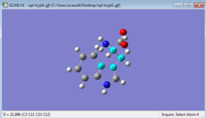
Optimization calculations are not too difficult. However, challenges can arise as can many different results. I did an optimization on three different conformations of tryptophan that I created by changing one of many dihedral angles in the molecule (Two C’s in pentagon across from N, the next Carbon in substituent chain, and the next Carbon which was bonded to NH2).

image

I used angles of 0, 135, and 180 degrees. Using the “broom”/”sweep” button on GaussView, I was able to return each configuration to a more energetically favorable conformation near those angles (21.99, -158.0, 41.5, respectively). However, they were not all the same since these angles are quite far from one another. When I performed an optimization calculation, each gave very similar energies (within 2 kJ/mol; in fact the first and third configuration were the same up to the fourth decimal place), but ranged in their change in energy from the “swept” conformation.

Here comes the issue. One calculation would not run (B3LYP/6-31G). It failed three times, each 15 minute long trials. The error message overall read “Error with lnk1e” followed by another line of error (which I do not remember). This suggested that the error arose because the “redundant internal coordinates” of this optimization were not working. So, one method to fix this issue would be to run the calculation starting from the current coordinates in the checkpoint file to redefine the internal coordinates and essentially bypass the error. Yet, in one of the output images, one C-C bond was essentially broken which shows that in its attempt to optimize the energy of tryptophan, GaussView felt that these two atoms needed to be further apart (about 1.75 Angstroms) than a normal C-C bond (1.54 A). This is not a scenario that should be repeated so the method of starting with new coordinates from the checkpoint file would not be effective. Therefore, instead we decided to use Cartesian coordinates which required adding “opt=cartesian” into the keywords of the route line.

Although a cartesian calculation takes much longer, I was able to find the proper energy of the optimized molecule.


1 Comment

Filed under chemistry